Gimy: 2020

2020年11月22日星期日

SQLite

create table [table_name] (SN INTEGER PRIMARY KEY AUTOINCREMENT)

select * from sqlite_master

2020年10月29日星期四

JS 筆記

parseInt("abc")            // 傳回NaN
parseInt("123abc")         // 傳回 123
parseInt("abc123")         // 傳回 NaN
parseInt("      123abc")   // 傳回 123

parseFloat("20");            //傳回20
parseFloat("30.00");         //傳回30
parseFloat("10.68");         //傳回10.68
parseFloat("12 22 32");      //傳回12
parseFloat("        80   "); //傳回80
parseFloat("378abc");        //傳回378
parseFloat("abc378");        //傳回NaN

Number(true);               //傳回1
Number(false);              //傳回0
Number(new Date());         //傳回1970/1/1到現在的毫秒數
Number("123");              //傳回123
Number("123 456");          //傳回NaN

2020年7月18日星期六

背景執行 gunicorn

安裝

sudo pip install gunicorn

背景執行

sudo gunicorn -w 1 -b 0.0.0.0:80 run:app --daemon

結束

查PID

ps -ef | grep gunicorn

sudo kill -9 12705

2020年7月16日星期四

pip

pip install opencv-python

pip install tqdm

2020年7月2日星期四

資料前處理

from sklearn.preprocessing import MinMaxScaler

scaler = MinMaxScaler()

df["population_density"] = scaler.fit_transform(df["population_density"].values.reshape(-1, 1))

2020年6月20日星期六

python df heatmap

heatmap = df[["city","class"]]

heatmap["cnt"] = 1

heatmap = heatmap.groupby(["city","class"]).sum().unstack().fillna(0)

2020年6月19日星期五

sigmoid

def sigmoid(X): # define activation: sigmoid

output = 1 / (1 + np.exp(-X))

return output

def sigmoid_gradient(X):

output = sigmoid(X)*(1-sigmoid(X))

return output

def softmax(X): # define activation: softmax

return np.exp(X) / np.sum(np.exp(X), axis=1, keepdims=True)

def cross_entropy(p, q):

epsilon = 1e-15

H = 0

for i in range(len(p)):

H += -p[i]*np.log(q[i]+epsilon)

H = H.sum()/p.shape[0]

return H

from tensorflow import keras

# 做 One-hot encoding

y = keras.utils.to_categorical(array)

2020年6月18日星期四

SQL (MySQL)

查詢table更新時間

select UPDATE_TIME FROM information_schema.TABLES where TABLE_NAME='{}'

SHOW VARIABLES LIKE '%group_concat%';

SET GLOBAL group_concat_max_len=102400;

SET SESSION group_concat_max_len=102400;

ON DUPLICATE KEY UPDATE

ALTER TABLE Persons ADD UNIQUE (Id_P)

GROUP_CONCAT()

update update_test A inner join (select PAY_DATE,sum(EXPENSE) as U1,max(EXPENSE) as U2 from expense where PAY_DATE >= '2020/4/1' group by PAY_DATE) B on A.PAY_DATE=B.PAY_DATE set A.SUM_PAY=B.U1,A.MAX_PAY=B.U2;

數字轉字串
CONVERT(1,CHAR)

修改表格名
ALTER TABLE `原表格名` RENAME TO `新表格名`

改欄位名稱
ALTER TABLE `表格名` CHANGE COLUMN `舊欄位名` `新欄位名` 欄位類型
ALTER TABLE mfg_skill CHANGE COLUMN STAGE DEPT varchar(6)

2020年6月11日星期四

GitLab

Git global setup

git config --global user.name "智銘 吳"
git config --global user.email "wugimy@gmail.com"

Create a new repository

git clone https://gitlab.aiacademy.tw/at091013/my-first-project.git
cd my-first-project
touch README.md
git add README.md
git commit -m "add README"
git push -u origin master

Existing folder

cd existing_folder
git init
git remote add origin https://gitlab.aiacademy.tw/at091013/my-first-project.git
git add .
git commit -m "Initial commit"
git push -u origin master

Existing Git repository

cd existing_repo
git remote rename origin old-origin
git remote add origin https://gitlab.aiacademy.tw/at091013/my-first-project.git
git push -u origin --all
git push -u origin --tags

2020年6月6日星期六

python 中央極限定理 CLT

import numpy as np

import matplotlib.pyplot as plt

#每次擲n次骰子取平均

n = 20

#執行t次

t = 10000

data = []

for i in range(0,t):

s = np.random.randint(1, 7, n)

data.append(s.mean())

# 直方圖

plt.hist(data,bins=20)

plt.show()

print("平均:",np.mean(data))

python xbgoost

import xgboost as xgb

from xgboost.sklearn import XGBClassifier

xgbc = XGBClassifier()

xgbc.fit(X_train, y_train)

pred = xgbc.predict(X_test)

from sklearn.metrics import accuracy_score

accuracy_score(pred,y_test)

2020年6月5日星期五

python RandomForest

from sklearn import datasets

iris = datasets.load_iris()

x = iris.data #feature

y = iris.target # Label

from sklearn.model_selection import train_test_split

X_train,X_test,y_train,y_test = train_test_split(x,y,test_size=0.3, random_state=88)

from sklearn.ensemble import RandomForestClassifier

#from sklearn.datasets import make_classification

clf = RandomForestClassifier(max_depth=2, random_state=0)

clf.fit(X_train, y_train)

pred = clf.predict(X_test)

from sklearn.metrics import accuracy_score

accuracy_score(pred,y_test)

my_function.py

def df_to_mysql(df,table_name):

import pyodbc

cn = pyodbc.connect('DRIVER={MySQL ODBC 8.0 ANSI Driver};SERVER=localhost;DATABASE=my_db;USER=;PASSWORD=;OPTION=3;')

cn.execute("truncate table " + table_name)

for row in df.values:

SQL = ""

for i in row:

if SQL == "":

SQL = "insert into " + table_name + " values ('" + str(i) + "'"

else:

SQL += ",'" + str(i) + "'"

SQL += ")"

#print(SQL)

cn.execute(SQL)

cn.commit()

cn.close()

return "df_to_mysql1 execute completed"

#執行前確認DaraFrame與DB Schema一致

from my_function import df_to_mysql

print(df_to_mysql(df,"iris"))

python training 資料準備 (以DataFrame匯入) KNN

# 一開始先被好資料(df格式)

# 決定切割欄位

cols = ["x1","x2","x3","x4"]

x = np.array(df[cols])

y = np.array(df["y"])

from sklearn.model_selection import train_test_split

X_train,X_test,y_train,y_test = train_test_split(x,y,test_size=0.3, random_state=88)

#使用KNN演算法

from sklearn.neighbors import KNeighborsClassifier

#從k=1開始測試

knn = KNeighborsClassifier(n_neighbors=1)

knn.fit(X_train,y_train)

pred = knn.predict(X_test)

#使用決策樹

from sklearn import tree

clf = tree.DecisionTreeClassifier()

clf = clf.fit(X_train,y_train)

tree.plot_tree(clf)

#pred = clf.predict(X_test)

#測試資料與預測資料比較

from sklearn.metrics import classification_report,confusion_matrix

print(confusion_matrix(y_test,pred))

print(classification_report(y_test,pred))

python dict 字典

countries = ['China', 'Japan', 'North Korea', 'South Korea', 'Taiwan', 'Thailand']

capitals = ['Beijing', 'Tokyo', 'Pyongyang', 'Seoul', 'Taipei', 'Bangkok']

#將list合併後轉成字典

d = dict(zip(countries,capitals))

#增加

d["United States"] = "Washington D.C."

#刪除

del d["Thailand"]

建立新字典，將舊字典的 key,value互換

new_dict = {}

for key,value in d.items():

new_dict[value]=key

修改

new_dict["Washington D.C."] = "US"

python list

list to dict 字典

countries = ['China', 'Japan', 'North Korea', 'South Korea', 'Taiwan', 'Thailand']

capitals = ['Beijing', 'Tokyo', 'Pyongyang', 'Seoul', 'Taipei', 'Bangkok']

d = dict(zip(countries,capitals))

2020年6月4日星期四

MySQL DATE_FORMAT() 函數日期時間

DATE_FORMAT(NOW(),'%Y-%m-%T')

格式	描述
%a	缩写星期名
%b	缩写月名
%c	月，数值
%D	带有英文前缀的月中的天
%d	月的天，数值(00-31)
%e	月的天，数值(0-31)
%f	微秒
%H	小时 (00-23)
%h	小时 (01-12)
%I	小时 (01-12)
%i	分钟，数值(00-59)
%j	年的天 (001-366)
%k	小时 (0-23)
%l	小时 (1-12)
%M	月名
%m	月，数值(00-12)
%p	AM 或 PM
%r	时间，12-小时（hh:mm:ss AM 或 PM）
%S	秒(00-59)
%s	秒(00-59)
%T	时间, 24-小时 (hh:mm:ss)
%U	周 (00-53) 星期日是一周的第一天
%u	周 (00-53) 星期一是一周的第一天
%V	周 (01-53) 星期日是一周的第一天，与 %X 使用
%v	周 (01-53) 星期一是一周的第一天，与 %x 使用
%W	星期名
%w	周的天（0=星期日, 6=星期六）
%X	年，其中的星期日是周的第一天，4 位，与 %V 使用
%x	年，其中的星期一是周的第一天，4 位，与 %v 使用
%Y	年，4 位
%y	年，2 位

python 引用 py

a.py

name="weiwei"

age=18

def introduction():

print "hi everyone, I'm",name,",",age,"years ago!"

b.py

from mei import introduction

introduction()

2020年6月2日星期二

python 迴歸

import numpy as np

import matplotlib.pyplot as plt

#自訂x,y

x = np.array([1,2,3,4,5])

y = np.array([2,5,7,8,10])

#==========

# 散佈圖 + 迴歸

fig, ax = plt.subplots(figsize=(8, 4))

ax.scatter(x, y)

m, c = np.polyfit(x, y, 1) # 使用 Numpy 的 polyfit，參數 1 代表一維，算出 fit 直線斜率

ax.plot(x, m * x + c) # 使用 y = m * x + c 斜率和常數匯出直線

fig.suptitle('Scatter with regression')

plt.show()

#==========

predict = lambda x: m * x + c

print(predict(5))

2020年5月30日星期六

python 物件 class

class Polygon:

def __init__(self,*p):

self.p = p

def __repr__(self):

return perimeter()

def __str__(self):

return "perimeter is " + "{:>3.2f}".format(self.perimeter())

def perimeter(self):

p = self.p

#計算兩點距離(X1-X2)平方+(Y1-Y2)平方，開根號

i = len(p) - 1

d = ((p[0][0] - p[i][0]) ** 2 + (p[0][1] - p[i][1]) ** 2) ** 0.5

for i in range(1,len(p)):

d += ((p[i][0] - p[i-1][0]) ** 2 + (p[i][1] - p[i-1][1]) ** 2) ** 0.5

return d

triangle = Polygon((0,0), (3,0), (0,4))

diamond = Polygon((-1,0), (0,-1), (1,0), (0,1))

print(triangle.perimeter())

print(diamond.perimeter())

print(triangle)

print(diamond)

2020年5月29日星期五

python 信賴區間

import numpy as np

import scipy.stats as stats

# 估計 95% 信心水準下，老年人每星期看電視平均時間的信賴區間？

# alpha = 0.05

# 假設樣本平均時間的抽樣分配服從常態分佈: xbar ~ N(mu_xbar, sigma_xbar)

# 抽樣人數 n = 100 ; 樣本平均時間 xbar = 21.2 小時

# 母體看電視時間的標準差 sigma = 8 小時

def Interval_estimation(n, xbar, sigma, alpha):

# standard error of the mean:

se = sigma / np.sqrt(n)

# margin of error:

# Hint: Z_(0.05/2) for Two-tails

E = stats.norm.ppf(1 - alpha/2, loc=0, scale=1) * se

# (1 - alpha)% Confidence Interval of Population mean with Known Variance:

Interval = [xbar - E, xbar + E]

return Interval

Interval_estimation(n=100, xbar=21.2, sigma=8, alpha=0.05)

python pi 圓周率機率驗證

points = 10000

X = np.random.uniform(-1, 1, points)

Y = np.random.uniform(-1, 1, points)

# 落於圓內的點

inner_index = (X**2 + Y**2) <= 1

# 落於圓外的點

outer_index = ~inner_index

indices = (inner_index, outer_index)

X_inner, Y_inner = X[indices[0]], Y[indices[0]]

X_outer, Y_outer = X[indices[1]], Y[indices[1]]

[(X_inner, Y_inner), (X_outer, Y_outer)], indices

plt.scatter(X_inner, Y_inner,s=1,c='red',marker='o',alpha=0.8,label='C1')

plt.scatter(X_outer, Y_outer,s=1,c='blue',marker='o',alpha=0.8,label='C1')

plt.show()

percent = len(X_inner) / points

print("圈內機率:",percent)

print("圈內面積:",2 * 2 * percent)

print("實際pi:",np.pi)

print("gap:",np.pi - 4 * percent)

2020年5月28日星期四

asp rs 操作

'=======================

'var categories = ['c1','c2','c3','c4','c5','c6','c7','c8','c9','c10','c11'];

'var data_plan = [10,20,30,40,40,30,30,30,30,30,30];

'var data_act = [11,32,33,34,39,43,33,33,35,33,33];

'=======================

categories = ""

data_plan = ""

data_act = ""

While Not rs.EOF

categories = categories & "'" & rs(0) & "'"

data_plan = data_plan & "," & rs(1)

data_act = data_act & "," & rs(2)

rs.MoveNext

categories = "[" & mid(categories,2) & "]"

data_plan = "[" & mid(data_plan,2) & "]"

data_act = "[" & mid(data_act,2) & "]"

Wend

python dataframe df

#by欄位計數

df["ITEM_NAME"].value_counts()

#繪圖

df["EXPENSE"].value_counts().plot(kind="bar")

#補值

df.interpolate(method ='linear', limit_direction ='backward', limit = 1)

df合併(欄位) (以下兩種方式)

df1.join(df2)

df = pd.concat([df1, df2], axis=1)

#欄位list分割

df["RecentDelays"].apply(pd.Series)

#分割欄位

new = df.From_To.str.split("_",expand=True)

new.columns = ["From","To"]

df = df.join(new)

#刪除欄位

df.drop("From_To", axis = 1)

#修改欄位名稱

df.rename(columns={'a':'A'})

python 統計 scipy.stats

import numpy as np

arr = np.array([1,3,2,5,4,4,5,453,43,45,43,5])

print("平均:",arr.mean())

print("標準差:",arr.std())

print("變異數:",arr.var())

print(np.sort(arr))

print("中位數:",np.median(arr))

#四分之一位數

np.quantile(e,.25)

#眾數

v = [1,2,3,4,5,3,3,3,3,3,3,3,3,4,4,4,4,4,4,5]

print(np.argmax(np.bincount(v)))

#共變異數與相關係數

def cov(X, Y): # 嘗試手刻共變異數吧

s = 0

for i in range(0,len(X)):

s += (X[i] - X.mean()) * (Y[i] - Y.mean())

s /= (len(X) - 1)

return s

def cor(X, Y): # 嘗試手刻相關係數吧

s,sx,sy = 0,0,0

for i in range(0,len(X)):

s += (X[i] - X.mean()) * (Y[i] - Y.mean())

sx += (X[i] - X.mean()) ** 2

sy += (Y[i] - Y.mean()) ** 2

s /= (sx** 0.5) * (sy** 0.5)

return s

X = np.array([1,2,3,4,5,6])

Y = np.array([3,5,6,7,8,9])

#使用自訂函式

print(cov(X,Y))

print(cor(X,Y))

#使用Numpy

print(np.cov(X, Y))

print(np.corrcoef(X, Y))

#==========================================================

import scipy.stats as stats

# 請查看 P(X <= -1)，X服從標準常態分佈：

norm_cdf = stats.norm.cdf

print("P(X <= -1)=", norm_cdf(-1, loc=0, scale=1))

# 請畫出標準常態分佈的累積機率函數（CDF），範圍從-3至3：

x = np.linspace(-3, 3, 1000)

norm_cdf = stats.norm.cdf

plt.plot(x, norm_cdf(x, loc=0, scale=1))

plt.arrow(-1, 0, 0, norm_cdf(-1, loc=0, scale=1), head_width=0.02,

width=0.005, head_length=0.02, color='r')

plt.arrow(-1, norm_cdf(-1, loc=0, scale=1), -3, 0, head_width=0.02,

width=0.005, head_length=0.02, color='g')

plt.show()

# 請分別查看標準常態分佈的 2.5%, 50%, 97.5% 分位數：

norm_ppf = stats.norm.ppf

print("2.5% 分位數:", norm_ppf(0.025))

print("50% 分位數:", norm_ppf(0.5))

print("97.5% 分位數:", norm_ppf(0.975))

# 請以直方圖（histogram）觀察10000個標準常態分佈的隨機數結果：

norm_rvs = stats.norm.rvs(loc=0, scale=1, size=10000)

n, bins, patches = plt.hist(norm_rvs, 100, density=True, facecolor='green', alpha=0.6)

mu, sigma = 0, 1

x = np.linspace(stats.norm.ppf(0.0001), stats.norm.ppf(0.9999), 101)

y = stats.norm.pdf(bins)

l = plt.plot(bins, y, 'r--', linewidth=2)

plt.xlabel('norm_rvs')

plt.ylabel('Probability')

plt.title(r'$\mathrm{Histogram\ of\ Symmetric\ Distribution:}\ \mu=0,\ \sigma=1$')

plt.show()

#==========================================================

# 隨機抽樣(random sampling):

s0 = np.random.choice([1, 2, 3, 4, 5], 5, replace=False)

# 請利用隨機抽樣的方法，將20個樣本隨機分派至2種不同的群組：

s1 = np.random.choice(2, 20, replace=True)

# 請利用隨機抽樣的方法，從20個樣本中，隨機抽取10個子樣本分派至群組1：

s2 = np.random.choice(20, 10, replace=False)

print(s0)

print(s1)

print(s2)

2020年5月27日星期三

AIA 20200527 python 小考

#第1題

cx = [1, 3, 5, 7, 2, 1, 8]

def less_than_5(array):

y = []

for i in array:

if i < 5:

y.append(i)

return y

print(less_than_5(x))

#第2題

factory1 = {"條件1" : 30, "條件2" : 10, "溫度容許值" : 20}

factory2 = {"條件1" : 48763, "條件3" : 75, "溫度容許值" : 60}

def dict_merge_with_bigger(Dict1, Dict2):

ND = Dict1

for key in Dict2:

if ND.get(key):

if Dict2[key] > ND[key]:

ND[key]=Dict2[key]

else:

ND[key]=Dict2[key]

return ND

print(dict_merge_with_bigger(factory1, factory2))

#第3題

#對python物件不熟(待補)

#第4題

def min_max(array):

min_arr = np.array([])

max_arr = np.array([])

for i in array.transpose():

min_arr = np.append(min_arr,min(i))

max_arr = np.append(max_arr,max(i))

return (arr - min_arr) / (max_arr - min_arr)

import numpy as np

arr = np.array(

[[1,3,5],

[4,5,6],

[7,8,9]]

)

min_max(arr)

#第5題

def grouped_mean(df, column_name, threshold):

dict1 = dict(df[df[column_name]<threshold].mean())

dict2 = dict(df[df[column_name]>=threshold].mean())

return (dict1,dict2)

import pandas as pd

data = {"height":[150,170,167,158,160],

"weight":[38,80,59,60,50],

"salary":[41, 15, 30, 15, 25]}

df = pd.DataFrame(data)

grouped_mean(df, "weight", 60)

2020年5月26日星期二

指令

sudo systemctl stop dengonban.service

sudo app_v2/install.sh

sudo systemctl enable cloudsqlproxy.service

sudo systemctl start cloudsqlproxy.service

sudo systemctl start dengonban.service

sudo systemctl status dengonban.service

python seaborn 繪圖

import seaborn as sns

import pandas as pd

import matplotlib.pyplot as plt

speed = [4, 4, 7, 7, 8, 9, 10, 10, 10, 11, 11, 12, 12, 12, 12, 13, 13, 13, 13, 14, 14, 14, 14, 15, 15, 15, 16, 16, 17, 17, 17, 18, 18, 18, 18, 19, 19, 19, 20, 20, 20, 20, 20, 22, 23, 24, 24, 24, 24, 25]

dist = [2, 10, 4, 22, 16, 10, 18, 26, 34, 17, 28, 14, 20, 24, 28, 26, 34, 34, 46, 26, 36, 60, 80, 20, 26, 54, 32, 40, 32, 40, 50, 42, 56, 76, 84, 36, 46, 68, 32, 48, 52, 56, 64, 66, 54, 70, 92, 93, 120, 85]

cars_df = pd.DataFrame(

{"speed": speed,

"dist": dist

}

)

# 散佈圖 (Scatter plot)

sns.jointplot(x = "speed", y = "dist", data = cars_df)

# 線圖（Line plot)

sns.factorplot(data = cars_df, x="speed", y="dist", ci = None)

# 長條圖（Bar plot）

sns.countplot(x = "speed", data = cars_df)

normal_samples = np.random.normal(size = 100000) # 生成 100000 組標準常態分配（平均值為 0，標準差為 1 的常態分配）隨機變數

# 直方圖 Histogram

sns.distplot(normal_samples)

# 盒鬚圖 Box plot

sns.boxplot(normal_samples)

import seaborn as sns

ax = sns.scatterplot(x="x1", y="x2", hue="NY", data=df)

ax = sns.boxplot(x="NY", y="x1", data=df)

python matplotlib 繪圖

# 引入模組

import numpy as np

import pandas as pd

import matplotlib.pyplot as plt

x = pd.period_range(pd.datetime.now(), periods=200, freq='d')

x = x.to_timestamp().to_pydatetime()

# 產生三組，每組 200 個隨機常態分布元素

y = np.random.randn(200, 3).cumsum(0)

plt.plot(x, y)

plt.show()

#==========

#線圖

x = np.array([1, 2, 3])

y1 = np.array([1, 2, 3])

y2 = np.array([10, 20, 30])

plt.figure(figsize=(8,4))

plt.plot(x,y1,label="line-1",color="red",linewidth=2)

# b--粗體虛線

plt.plot(x,y2,"b--",label="line-2")

plt.xlabel("x label")

plt.ylabel("y label")

plt.title("PyPlot First Example")

#plt.ylim(-1.2,1.2)

plt.legend()

plt.show()

#==========

# 長條圖

labels = ['Physics', 'Chemistry', 'Literature', 'Peace']

foo_data = [3, 6, 10, 4]

bar_width = 0.5

xlocations = np.array(range(len(foo_data))) + bar_width

plt.bar(xlocations, foo_data, width=bar_width)

plt.title('Stock Price')

plt.show()

# 直方圖

normal_samples = np.random.normal(size=100) # 生成 100 組標準常態分配（平均值為 0，標準差為 1 的常態分配）隨機變數

plt.hist(normal_samples)

plt.show()

#==========

# 散佈圖 + 迴歸

num_points = 100

gradient = 0.5

x = np.array(range(num_points))

y = np.random.randn(num_points) * 10 + x * gradient

fig, ax = plt.subplots(figsize=(8, 4))

ax.scatter(x, y)

m, c = np.polyfit(x, y, 1) # 使用 Numpy 的 polyfit，參數 1 代表一維，算出 fit 直線斜率

ax.plot(x, m * x + c) # 使用 y = m * x + c 斜率和常數匯出直線

fig.suptitle('Scatter with regression')

plt.show()

#==========

# 圓餅圖

labels = ['A','B','C','D','E']

data = np.random.randint(1, 11, 5) # 生成

x = np.arange(len(data))

plt.pie(data, labels=labels, autopct='%1.1f%%')

plt.show()

#==========

# 盒鬚圖

normal_examples = np.random.normal(size = 100) # 生成 100 組標準常態分配（平均值為 0，標準差為 1 的常態分配）隨機變數

plt.boxplot(normal_examples)

plt.show()

# 把圖儲存，要放在plt.show()之前

plt.savefig("C:/savefig/hist.png")

2020年5月23日星期六

highcharts formatter

plotOptions: {

column: {

grouping: false,

shadow: false,

borderWidth: 0

line: {

dataLabels: {

enabled: true,

//format: '{y:.1f}'

formatter: function() {

return '<b>'+ Highcharts.numberFormat(this.y*100, 2) +'%</b><br/>';

}

2020年5月22日星期五

python LCS (Longest Common SubSequence) 共同字串

#Longest Common SubSequence

import numpy as np

S1="abcdefg"

S2="abzzcdzzefg"

L1 = list(S1)

L2 = list(S2)

#補零作為起始

L1.insert(0,"0")

L2.insert(0,"0")

A = np.zeros((len(L1), len(L2)), dtype=np.int)

#初始值

for i in range(0,len(L1)):

A[i,0] = -i

for j in range(0,len(L2)):

A[0,j] = -j

#計算距離矩陣

for i in range(1,len(L1)):

for j in range(1,len(L2)):

if L1[i] == L2[j]:

A[i,j] = A[i-1,j-1] + 2

else:

A[i,j] = max(A[i-1,j-1],A[i,j-1],A[i-1,j]) - 1

#回溯字串

i = len(L1)-1

j = len(L2)-1

LCS1 = ""

LCS2 = ""

while i > 0 and j > 0:

#左上

if A[i-1,j-1] >= max(A[i,j-1],A[i-1,j]):

LCS1 = L1[i] + LCS1

LCS2 = L2[j] + LCS2

i = i - 1

j = j - 1

#左

elif A[i,j-1] >= A[i-1,j]:

LCS1 = "-" + LCS1

LCS2 = L2[j] + LCS2

j = j - 1

#上

else:

LCS1 = L1[i] + LCS1

LCS2 = "-" + LCS2

i = i - 1

while i > 0:

LCS1 = L1[i] + LCS1

LCS2 = "-" + LCS2

i = i - 1

print("輸入的字串")

print(S1)

print(S2)

print("輸出的字串")

print(LCS1)

print(LCS2)

print("共同的字串")

for i in range(0,len(LCS1)):

if LCS1[i] == LCS2[i]:

print(LCS1[i],end="")

python numpy

import numpy as np

#array

x = np.array([1, 2, 3])

#產生隨機整數亂數(最小值,最大值,個數)

data = np.random.randint(1, 11, 10) # 生成10個1~10的亂數

python Fibonacci 費氏級數

def fib_generator(n):

L = [0,1]

if n <= 1:

return L[n]

else:

for i in range(2,n+1):

f = L[i-2]+L[i-1]

L.append(f)

return L

print(fib_generator(10))

python set 集合

s1 = {-3,-2,-1,0,1,2,3,4,5}

s2 = {1,2,3,4,5,6,7,8}

print("交集",s1 & s2)

print("聯集",s1 | s2)

print("差集",s1 - s2)

python 氣泡排序

L = [56, 81, 82, 79, 85, 45, 99, 49, 93, 27, 18, 54, 19, 32]

#氣泡排序 for i in range(0,len(L)-1): for j in range(1,len(L)-i): if L[j-1] > L[j]: #互換 L[j],L[j-1] = L[j-1],L[j] print(L)

python df to json

#force_ascii=False -> 轉中文

json = df.to_json(orient='records',force_ascii=False)

#存檔

f = open('C:/json/news.json','w')

f.write(json)

import json

# Reading data back

with open('C:/json/news.json', 'r') as f:

data = json.load(f)

#data(list)轉回df

df = pd.DataFrame(data)

python df merge (left outer join)

#left outer join
df = df1.merge(df2, on=['MFG_DAY','EQP_ID'], how='left')

python pandas (list to DataFrame)

import pandas as pd

baby_name = ["A","B","C"]

bavy_birth = [100,200,300]

baby_ds = list(zip(baby_name,bavy_birth))

baby_df = pd.DataFrame(baby_ds,columns=['name','birth'])

baby_df

python 函數 def

def multiply(m, n):

return m * n

print(multiply(2, 3))

python 字串處理

#####################################

s="0123456789"

print(s[:5])

print(s[:5:2])

s.find("2") # 找字

#####################################

# 印出三角*

for i in range(0,10):

for j in range(0,i+1):

print("*",end="") # 不換行

print("")

#####################################

#Longest Common SubSequence

import numpy as np

S1="abcdefg"

S2="abzzcdzzefg"

L1 = list(S1)

L2 = list(S2)

#補零作為起始

L1.insert(0,"0")

L2.insert(0,"0")

A = np.zeros((len(L1), len(L2)), dtype=np.int)

#初始值

for i in range(0,len(L1)):

A[i,0] = -i

for j in range(0,len(L2)):

A[0,j] = -j

#計算距離矩陣

for i in range(1,len(L1)):

for j in range(1,len(L2)):

if L1[i] == L2[j]:

A[i,j] = A[i-1,j-1] + 2

else:

A[i,j] = max(A[i-1,j-1],A[i,j-1],A[i-1,j]) - 1

#回溯字串

i = len(L1)-1

j = len(L2)-1

LCS1 = ""

LCS2 = ""

while i > 0 and j > 0:

#左上

if A[i-1,j-1] >= max(A[i,j-1],A[i-1,j]):

LCS1 = L1[i] + LCS1

LCS2 = L2[j] + LCS2

i = i - 1

j = j - 1

#左

elif A[i,j-1] >= A[i-1,j]:

LCS1 = "-" + LCS1

LCS2 = L2[j] + LCS2

j = j - 1

#上

else:

LCS1 = L1[i] + LCS1

LCS2 = "-" + LCS2

i = i - 1

while i > 0:

LCS1 = L1[i] + LCS1

LCS2 = "-" + LCS2

i = i - 1

print("輸入的字串")

print(S1)

print(S2)

print("輸出的字串")

print(LCS1)

print(LCS2)

print("共同的字串")

for i in range(0,len(LCS1)):

if LCS1[i] == LCS2[i]:

print(LCS1[i],end="")

2020年5月19日星期二

python MySQL

import pyodbc

import pandas as pd

cn = pyodbc.connect('DRIVER={MySQL ODBC 8.0 ANSI Driver};SERVER=localhost;DATABASE=my_db;USER=root;PASSWORD=xxxx;OPTION=3;')

SQL = "select * from expense"

df = pd.read_sql(SQL, cn)

cn.close()

2020年5月13日星期三

python 判斷是否為數字

def is_number(str):

try:

# 因為使用float有一個例外是'NaN'

if str=='NaN':

return False

float(str)

return True

except ValueError:

return False

print(is_number("123"))

str為字串s為字串

str.isalnum() 所有字元都是數字或者字母

str.isalpha() 所有字元都是字母

str.isdigit() 所有字元都是數字

str.isspace() 所有字元都是空白字元、t、n、r

2020年5月12日星期二

python 日期週的使用

import datetime

from_date = (datetime.date.today()-datetime.timedelta(days=1)).strftime('%Y-%m-%d')

#週的第一天

#python星期定義為一到日:0~6

#日期寫法:datetime.datetime(2020, 5, 11)

today = datetime.date.today()

#週的第幾天(以0起算)

week_days = (today.weekday()+1) % 7

week_start = today - datetime.timedelta(days=week_days)

print(week_start)

delta = datetime.timedelta(days=7)

MFG_DAY = week_start - delta * 10

for i in range(0,11):

print((MFG_DAY + delta * i).strftime('%Y/%m/%d'),"第",(MFG_DAY + delta * i).isocalendar()[1],"週")

2020年5月10日星期日

python 檔案處理

#複製檔案
import shutil
source = "//10.88.39.45/mfg/AI_Picture/weilunwu/test1/aaa.txt"
target = "//10.88.39.45/mfg/AI_Picture/weilunwu/test2/aaa.txt"
shutil.copyfile(source,target)

2020年4月24日星期五

ORA-12154: TNS: 無法解析指定的連線 ID

最近朋友使用 EF 連到 Oracle ，在本機上執行的好好的。

將程式部署到另一台機器就發生了「ORA-12154: TNS: 無法解析指定的連線 ID」的錯誤，如下，

環境變數也都有加入 TNS_ADMIN 呀!

後來只好在 web.config 中再加入 TNS_ADMIN 的設定，如下，

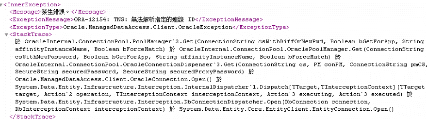
<configuration>
  <oracle.manageddataaccess.client>
    <version number="*">
      <settings>
        <setting name="TNS_ADMIN" value="C:\oracle\network\admin**請調整機器上的Path "/>
      </settings>
    </version>
  </oracle.manageddataaccess.client>
</configuration>

2020年3月26日星期四

python train model

from sklearn import preprocessing
import numpy as np
import matplotlib.pyplot as plt
from sklearn import datasets
from sklearn.svm import SVC

cancer = datasets.load_breast_cancer()
x = cancer.data #feature
y = cancer.target # Label

from sklearn.model_selection import train_test_split
X_train,X_test,y_train,y_test = train_test_split(x,y,test_size=0.3, random_state=88)
# 建立要學習的模型
svm = SVC(kernel='linear', random_state=0)
#訓練==>
svm.fit(X_train, y_train)
y_pred = svm.predict(X_test)

print(y_pred)
print(y_test)
from sklearn.metrics import accuracy_score
accuracy_score(y_pred,y_test)

2020年3月18日星期三

jQuery ajax 定期更新跳訊息

<!DOCTYPE html>
<html>
<head>
<title></title>

<script src="https://code.jquery.com/jquery-3.4.1.min.js" type="text/javascript" ></script>
<script src="notice.js" type="text/javascript" ></script>
</head>
<body>
HELLO
<script>
$(document).ready(function () {
setInterval("startRequest()",1000);
});
function startRequest()
{
htmlobj=$.ajax({url:"ajax_info.txt",async:false});
$("#date").text((new Date()).toString());
$("#myDiv").html(htmlobj.responseText);

var dt = new Date();
if (dt.getSeconds()==0) {
pop();
}

}

function pop() {
var returnMsg = "內容";
$.show("標題",returnMsg,10000);
}

</script>

<div id="date">aaa</div>
<div id="myDiv"><h2>AJAX</h2></div>
</body>
</html>

2020年3月10日星期二

python to_txt

import pyodbc
import pandas as pd # 引用套件並縮寫為 pd

cnxn = pyodbc.connect("DRIVER={MySQL ODBC 8.0 Unicode Driver}; SERVER=localhost; PORT=3306;DATABASE=my_db; UID=root; PASSWORD=gimy0710;OPTION=3;CHARSET=UTF8;")
SQL = "SELECT * FROM expense where PAY_DATE > '2020/1/1' order by PAY_DATE desc"
file_name = "test.txt"

df = pd.read_sql(SQL, cnxn)
cnxn.close()

txt = ""
for row in df.columns:
txt = txt + row + "|"
txt = txt + "\n"

for row in df.values:
for i in range(0,len(row)):
txt = txt + str(row[i]) + "|"
txt = txt + "\n"
#print(txt)
f = open(file_name,'w')
f.write(txt)
f.close()

2020年2月26日星期三

python to_csv

###############################

import pandas as pd

df = pd.read_csv("C:/data/data.csv")

df.to_csv("C:/data/data_output.csv")

2020年2月22日星期六

highcharts

<!DOCTYPE html>
<html>
<head>

<style>
.highcharts-figure, .highcharts-data-table table {
min-width: 360px;
max-width: 800px;
margin: 1em auto;
}

.highcharts-data-table table {
font-family: Verdana, sans-serif;
border-collapse: collapse;
border: 1px solid #EBEBEB;
margin: 10px auto;
text-align: center;
width: 100%;
max-width: 500px;
}
.highcharts-data-table caption {
padding: 1em 0;
font-size: 1.2em;
color: #555;
}
.highcharts-data-table th {
font-weight: 600;
padding: 0.5em;
}
.highcharts-data-table td, .highcharts-data-table th, .highcharts-data-table caption {
padding: 0.5em;
}
.highcharts-data-table thead tr, .highcharts-data-table tr:nth-child(even) {
background: #f8f8f8;
}
.highcharts-data-table tr:hover {
background: #f1f7ff;
}
</style>

</head>
<body>

<script src="https://code.highcharts.com/highcharts.js"></script>
<script src="https://code.highcharts.com/modules/series-label.js"></script>
<script src="https://code.highcharts.com/modules/exporting.js"></script>
<script src="https://code.highcharts.com/modules/export-data.js"></script>
<script src="https://code.highcharts.com/modules/accessibility.js"></script>

<figure class="highcharts-figure">
<div id="container"></div>
<p class="highcharts-description">
Basic line chart showing trends in a dataset. This chart includes the
<code>series-label</code> module, which adds a label to each line for
enhanced readability.
</p>
</figure>

<script>

var data_name = ['data0','data1'];
var data0 = [49.9, 71.5, 106.4, 129.2, 144.0, 176.0, 135.6, 148.5, 216.4, 194.1, 95.6, 54.4];
var data1 = [49.9, 71.5, 106.4, 129.2, 144.0, 176.0, 135.6, 148.5, 216.4, 194.1, 95.6, 54.4];

var ratio = new Array(data0.length);
for(i=0;i < data0.length;i++){
ratio[i] = data0[i] / (data0[i] + data1[i]);
ratio[i] = ratio[i] * 100;
}

Highcharts.chart('container', {
chart: {
zoomType: 'xy'
},
title: {
text: 'Average Monthly Temperature and Rainfall in Tokyo'
},
subtitle: {
text: 'Source: WorldClimate.com'
},
xAxis: [{
categories: ['Jan', 'Feb', 'Mar', 'Apr', 'May', 'Jun',
'Jul', 'Aug', 'Sep', 'Oct', 'Nov', 'Dec'],
crosshair: true
}],
yAxis: [{ // Primary yAxis
labels: {
format: '{value}°C',
style: {
color: Highcharts.getOptions().colors[1]
}
},
title: {
text: 'Temperature',
style: {
color: Highcharts.getOptions().colors[1]
}
}
}, { // Secondary yAxis
title: {
text: 'Ratio (%)',
style: {
color: Highcharts.getOptions().colors[0]
}
},
labels: {
format: '{value} mm',
style: {
color: Highcharts.getOptions().colors[0]
}
},
opposite: true
}],
tooltip: {
shared: true
},
legend: {
layout: 'vertical',
align: 'left',
x: 120,
verticalAlign: 'top',
y: 100,
floating: true,
backgroundColor:
Highcharts.defaultOptions.legend.backgroundColor || // theme
'rgba(255,255,255,0.25)'
},

plotOptions: {
column: {
stacking: 'normal',
dataLabels: {
enabled: true
}
}
},

series: [
{
name: data_name[0],
type: 'column',

data: data0

},
{
name: data_name[1],
type: 'column',
data: data1

},
{
name: 'Ratio',
type: 'line',
yAxis: 1,
data: ratio
}]
});
</script>

</body>
</html>

2020年2月19日星期三

python-matplotlib

import matplotlib.pyplot as plt

plt.rcParams['font.sans-serif']=['SimHei'] #用來正常顯示中文標籤

四大圖表

CCRD

2020年2月11日星期二

load excel

import pandas as pd
df = pd.read_excel (r'D:\Python_Test.xlsx')
#for an earlier version of Excel, you may need to use the file extension of 'xls'
lines = df.values
cols = df.columns
for i in cols:
print(i)
for i in lines:
print(i)

requests

import requests
url = "https://www.books.com.tw/"
htmlfile = requests.get(url)
print(type(htmlfile))
print(htmlfile.text)

2020年11月22日 星期日

2020年10月29日 星期四

2020年7月18日 星期六

2020年7月16日 星期四

2020年7月2日 星期四

2020年6月20日 星期六

2020年6月19日 星期五

2020年6月18日 星期四

數字轉字串CONVERT(1,CHAR)

修改表格名ALTER TABLE `原表格名` RENAME TO `新表格名`

改欄位名稱ALTER TABLE `表格名` CHANGE COLUMN `舊欄位名` `新欄位名` 欄位類型ALTER TABLE mfg_skill CHANGE COLUMN STAGE DEPT varchar(6)

2020年6月11日 星期四

Git global setup

Create a new repository

Existing folder

Existing Git repository

2020年6月6日 星期六

2020年6月5日 星期五

2020年6月4日 星期四

2020年6月2日 星期二

2020年5月30日 星期六

2020年5月29日 星期五

2020年5月28日 星期四

2020年5月27日 星期三

2020年5月26日 星期二

2020年5月23日 星期六

2020年5月22日 星期五

2020年5月19日 星期二

2020年5月13日 星期三

2020年5月12日 星期二

2020年5月10日 星期日

2020年4月24日 星期五

2020年3月26日 星期四

2020年3月18日 星期三

2020年3月10日 星期二

2020年2月26日 星期三

2020年2月22日 星期六

2020年2月19日 星期三

2020年2月11日 星期二

2020年11月22日星期日

2020年10月29日星期四

2020年7月18日星期六

2020年7月16日星期四

2020年7月2日星期四

2020年6月20日星期六

2020年6月19日星期五

2020年6月18日星期四

數字轉字串
CONVERT(1,CHAR)

修改表格名
ALTER TABLE `原表格名` RENAME TO `新表格名`

改欄位名稱
ALTER TABLE `表格名` CHANGE COLUMN `舊欄位名` `新欄位名` 欄位類型
ALTER TABLE mfg_skill CHANGE COLUMN STAGE DEPT varchar(6)

2020年6月11日星期四

2020年6月6日星期六

2020年6月5日星期五

2020年6月4日星期四

2020年6月2日星期二

2020年5月30日星期六

2020年5月29日星期五

2020年5月28日星期四

2020年5月27日星期三

2020年5月26日星期二

2020年5月23日星期六

2020年5月22日星期五

2020年5月19日星期二

2020年5月13日星期三

2020年5月12日星期二

2020年5月10日星期日

2020年4月24日星期五

2020年3月26日星期四

2020年3月18日星期三

2020年3月10日星期二

2020年2月26日星期三

2020年2月22日星期六

2020年2月19日星期三

2020年2月11日星期二